FLARE made global attention affordable on million-point meshes by routing $N$ tokens through $M \ll N$ learned latent queries. Once trained, though, those $M$ queries are frozen: the same compression template serves every geometry, every boundary condition, and every flow field. FLARE++ keeps FLARE’s low-rank structure and linear cost, and lets the current input shape the queries that compress it.
This post walks through the idea. The paper is FLARE++: Low-rank attention with attention-synthesized routing (with Sri Datta Ganesh Bandreddi, Jessica Zhang, and Burak Kara), and the code is in FLARE.py. If you have not read the FLARE post, start there; this one builds directly on it.
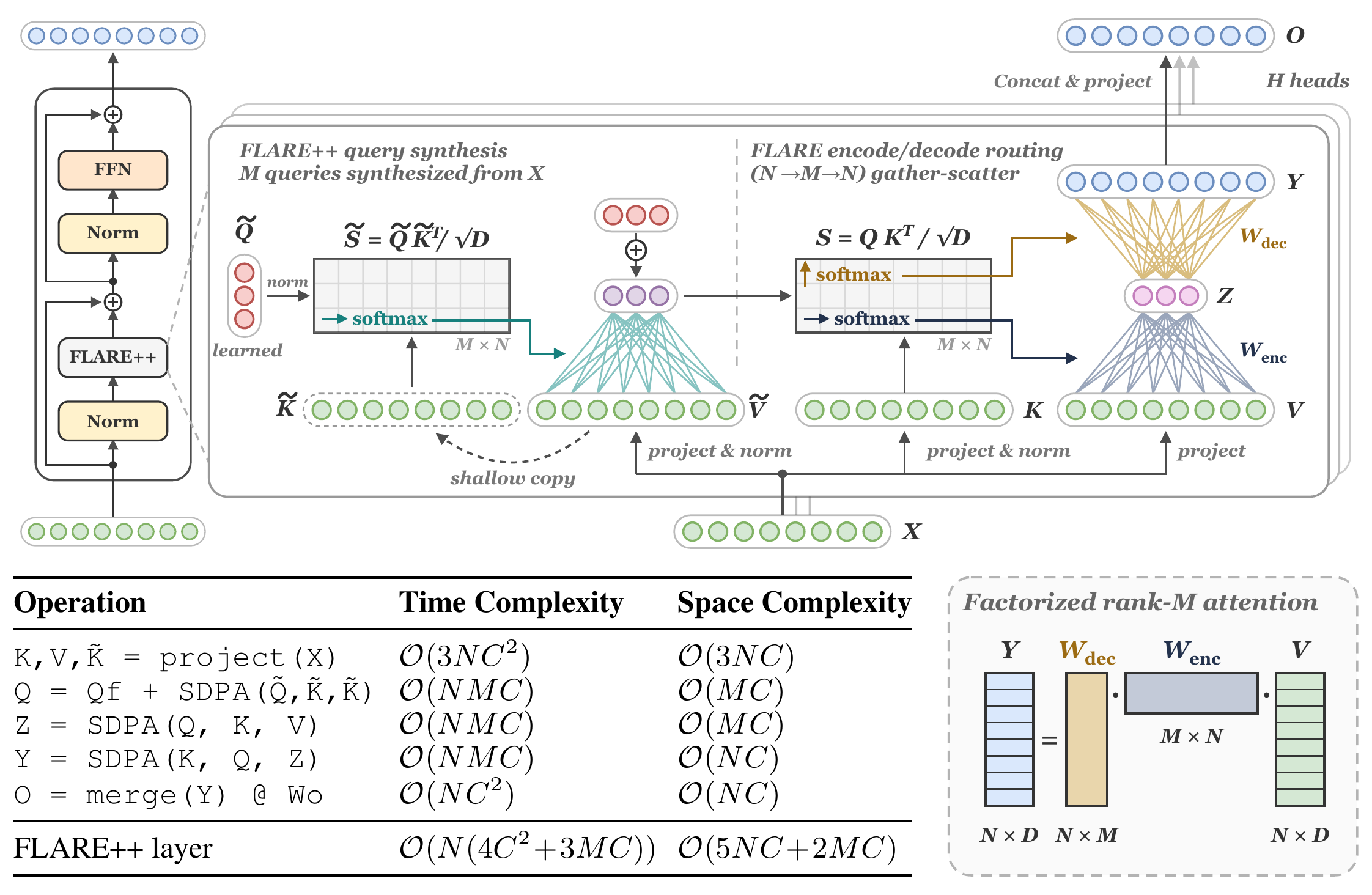
Recap: FLARE as a rank-$M$ attention operator
Full self-attention lets each of $N$ points attend to every other at $\mathcal{O}(N^2)$ cost. FLARE replaces the dense $N \times N$ score matrix with an encode–decode pair through $M$ latent routes. Each head owns a learned query set $Q_h \in \mathbb{R}^{M \times D}$, and keys and values come from the input:
$$ Z_h = \mathrm{SDPA}(Q_h, K_h, V_h), \qquad Y_h = \mathrm{SDPA}(K_h, Q_h, Z_h). $$The first call gathers $N$ tokens into $M$ latents; the second scatters them back. Together they apply an $N \times N$ mixing matrix $W_{\mathrm{dec},h} W_{\mathrm{enc},h}$ of rank at most $M$, which is never materialized because both calls are fused SDPA kernels. Cost is $\mathcal{O}(NM)$ per head.
The limitation: a fixed compression template
Latent-attention mixers such as Perceiver IO, the Transolver family, LNO, Set Transformer, Luna, and FLARE decide what to compress by dot-product matching the input tokens against something learned: latent query tokens, or projection weights. I call these addressing vectors the compression template.
In FLARE the template is the $M$ query vectors per head and layer. The routing weights do respond to the input, because the keys change. But the queries that define the template never see the field they are compressing. A car body, an airfoil, and a porous medium all get compressed against the same $M$ directions.
The other family of methods builds the template from the data: Nyströmformer’s segment means, Agent Attention’s pooled queries, UPT’s supernodes, AB-UPT’s sampled anchors. These do change per input, but latent $m$ has no identity across inputs: anchor 17 on one mesh has nothing to do with anchor 17 on another. And segment means or pooling lean on token order or grids that unstructured meshes do not have.
FLARE++ tries to get both: a learned template with persistent identities, adapted to each input.
FLARE++: synthesizing the routing queries
The key observation is that FLARE already has an operator that summarizes $N$ tokens into $M$ vectors: its own encoder. So we run it one extra time, with learned seeds $\widetilde{Q}_h$ as queries, and use the output as a correction to the routing queries.
Step 1: synthesize. Project the input to synthesis keys, normalize them, and share them as values:
$$ \widetilde{K}_h = \mathcal{N}_0(X \widetilde{W}_{K,h}), \qquad \widetilde{V}_h = \widetilde{K}_h, $$$$ Q^{\mathrm{d}}_h(X) = \mathrm{SDPA}\big(\mathcal{N}_a(\widetilde{Q}_h),\, \widetilde{K}_h,\, \widetilde{V}_h\big) \in \mathbb{R}^{M \times D}. $$Each row of $Q^{\mathrm{d}}_h$ is a convex combination of unit-RMS rows, so its RMS is at most 1. The correction is bounded without being renormalized, and its magnitude carries information: it is large when the attended features agree and small when they cancel.
Step 2: gate onto a learned reference.
$$ Q_h(X) = \mathcal{N}_0(Q^{\mathrm{f}}_h) + g_h\, Q^{\mathrm{d}}_h(X), \qquad g_h = \sigma(\gamma_h) \in (0,1). $$The fixed reference $Q^{\mathrm{f}}_h$ plays the role of FLARE’s queries and gives a common routing basis. The synthesized term deforms it toward the current field. As $g_h \to 0$ you recover fixed-query FLARE.
Step 3: route as before.
$$ Z_h = \mathrm{SDPA}(Q_h(X), K_h, V_h), \qquad Y_h = \mathrm{SDPA}(K_h, Q_h(X), Z_h). $$For each fixed input the mixing matrix is still rank $\le M$. But now the current field decides the queries used for both gathering and dispatch. Because each correction aggregates over the whole field, changing one region can change how every token in the block is addressed.
One attention call builds the routes; two more move values along them. That is the whole change. The backbone keeps the same depth, width, and residual structure; every added component (synthesis projection, seeds, gate, per-head norms) acts only through the routing scores $Q_h K_h^\top$.
In code
Here is a complete, runnable PyTorch implementation of the mixer and the residual block around it.
Each step is labeled with the matching row of the cost table in the figure above.
It needs PyTorch 2.4 or later for nn.RMSNorm.
import torch
import torch.nn as nn
import torch.nn.functional as F


class FLAREPPMixer(nn.Module):
    """FLARE++ token mixer. X: [B, N, C] -> O: [B, N, C], with C = H * D."""

    def __init__(self, C: int, H: int = 8, M: int = 64, gate_init: float = 0.25):
        super().__init__()
        assert C % H == 0
        self.H, self.D = H, C // H
        D = self.D

        # projections for K, V, K~, and the output
        self.Wk = nn.Linear(C, C)
        self.Wv = nn.Linear(C, C)
        self.Wk_syn = nn.Linear(C, C)
        self.Wo = nn.Linear(C, C)

        # learned latents: M per head
        self.Q_seed = nn.Parameter(0.02 * torch.randn(H, M, D))  # Q~, synthesis seeds
        self.Q_fix = nn.Parameter(0.02 * torch.randn(H, M, D))   # Qf, fixed reference
        self.gate = nn.Parameter(torch.full((H,), gate_init))     # g_h = sigmoid(gate_h)

        # per-head RMSNorm: N_a has a learned scale, N_0 does not
        self.norm_seed = nn.RMSNorm(D, eps=1e-6)
        self.norm_k = nn.RMSNorm(D, eps=1e-6)
        self.norm0 = nn.RMSNorm(D, eps=1e-6, elementwise_affine=False)

    def heads(self, T):
        # [B, N, C] -> [B, H, N, D]
        B, N, _ = T.shape
        return T.view(B, N, self.H, self.D).transpose(1, 2)

    def forward(self, X):
        B, N, C = X.shape

        # K, V, K~ = project(X)
        K = self.norm_k(self.heads(self.Wk(X)))
        V = self.heads(self.Wv(X))
        Ks = self.norm0(self.heads(self.Wk_syn(X)))  # used as both keys and values

        # Q = Qf + SDPA(Q~, K~, K~)
        Qs = self.norm_seed(self.Q_seed).expand(B, -1, -1, -1)
        Qd = F.scaled_dot_product_attention(Qs, Ks, Ks)          # [B, H, M, D]
        # gated sum in FP32, then cast back (matters under FP16/BF16 autocast)
        Qf = self.norm0(self.Q_fix).float()
        g = torch.sigmoid(self.gate).float().view(1, self.H, 1, 1)
        Q = (Qf + g * Qd.float()).to(X.dtype)                      # [B, H, M, D]

        # Z = SDPA(Q, K, V): gather N tokens into M latents
        Z = F.scaled_dot_product_attention(Q, K, V)                # [B, H, M, D]

        # Y = SDPA(K, Q, Z): scatter M latents back to N tokens
        Y = F.scaled_dot_product_attention(K, Q, Z)                # [B, H, N, D]

        # O = merge(Y) @ Wo
        return self.Wo(Y.transpose(1, 2).reshape(B, N, C))


class FLAREPPBlock(nn.Module):
    """Pre-norm residual block: X + FLARE++(Norm(X)), then X + FFN(Norm(X))."""

    def __init__(self, C: int, H: int = 8, M: int = 64, mlp_ratio: float = 2.0):
        super().__init__()
        self.norm1 = nn.RMSNorm(C, eps=1e-6)
        self.norm2 = nn.RMSNorm(C, eps=1e-6)
        self.mixer = FLAREPPMixer(C, H, M)
        self.ffn = nn.Sequential(
            nn.Linear(C, int(mlp_ratio * C)),
            nn.GELU(),
            nn.Linear(int(mlp_ratio * C), C),
        )

    def forward(self, X):
        X = X + self.mixer(self.norm1(X))
        X = X + self.ffn(self.norm2(X))
        return X


if __name__ == "__main__":
    block = FLAREPPBlock(C=128, H=8, M=64)
    X = torch.randn(2, 10_000, 128)  # 2 inputs, 10K points, 128 channels
    print(block(X).shape)            # torch.Size([2, 10000, 128])
Three fused SDPA calls, no custom kernel, no $N \times M$ matrix in memory.
The reference implementation, pdebench/models/flarepp.py, has the same structure; it adds weight initialization and the context-parallel encoder described below, and uses LayerNorm in place of RMSNorm for full-precision runs.
Why the normalization and the gate
The first version was the pure form: route with $Q^{\mathrm{d}}_h(X)$ alone. In FP32 it works essentially as well as the gated version. But the output of the synthesis call becomes the query of the routing calls, so the routes move while the encoder is still learning to use them. Early training is touchy, and in FP16 the pure form degraded and was hard to train.
Two things fixed that: RMS-normalizing every tensor that enters an attention score, and anchoring the synthesized queries to a fixed reference through the gate. With both, FLARE++’s FP16 error stays within 8% of its FP32 error at every depth we tried. It is worth being clear that the normalizations are not where the accuracy comes from: adding them to FLARE did not improve it, and the ungated synthesis variant gets roughly the same FP32 gain without them.
Cost
FLARE++ adds one projection ($\widetilde{K}$) and one SDPA call per block:
| Time per block | |
|---|---|
| FLARE | $\mathcal{O}(N(3C^2 + 2MC))$ |
| FLARE++ | $\mathcal{O}(N(4C^2 + 3MC))$ |
| Full self-attention | $\mathcal{O}(N^2 C)$ |
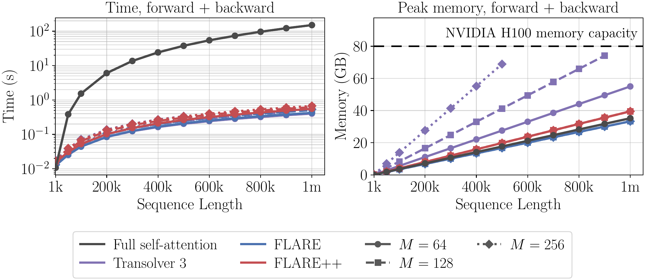
Both stay linear in $N$. The mixer arithmetic goes up by $4/3$ to $3/2$; measured end-to-end on one H100, FLARE++ costs $1.2$–$1.3\times$ FLARE’s step time and $1.18\times$ its peak memory, because the feed-forward network dilutes the mixer’s share.
Scaling past one GPU
Linear complexity does not make an 8M-cell mesh fit on one accelerator, because pointwise activations still grow with $N$. So we shard tokens across GPUs.
Because tokens only interact through $M$ latents, this turns out to be simple. Projections, norms, FFNs, and residuals are all local. The only global operation is the encoder, and that is exactly the case the blockwise / Ring Attention log-sum-exp merge was built for: each rank runs SDPA on its local tokens, returns a partial output $Z_r$ and log-normalizer $L_r$, and one all-reduce combines them,
$$ L = \log \sum_r \exp(L_r), \qquad Z = \sum_r \exp(L_r - L)\, Z_r. $$That equals the single-device encoder in exact arithmetic, and the message is $\mathcal{O}(HM(D+2))$ values per rank, independent of $N$. Decoding is then local, so the full token sequence is never gathered anywhere. FLARE++ calls the distributed encoder twice (once to synthesize $Q(X)$, once to gather $Z$). On up to four H100s, time and memory efficiencies stay at or above about $0.91$ and $0.95$.
Results
Standard PDE benchmarks
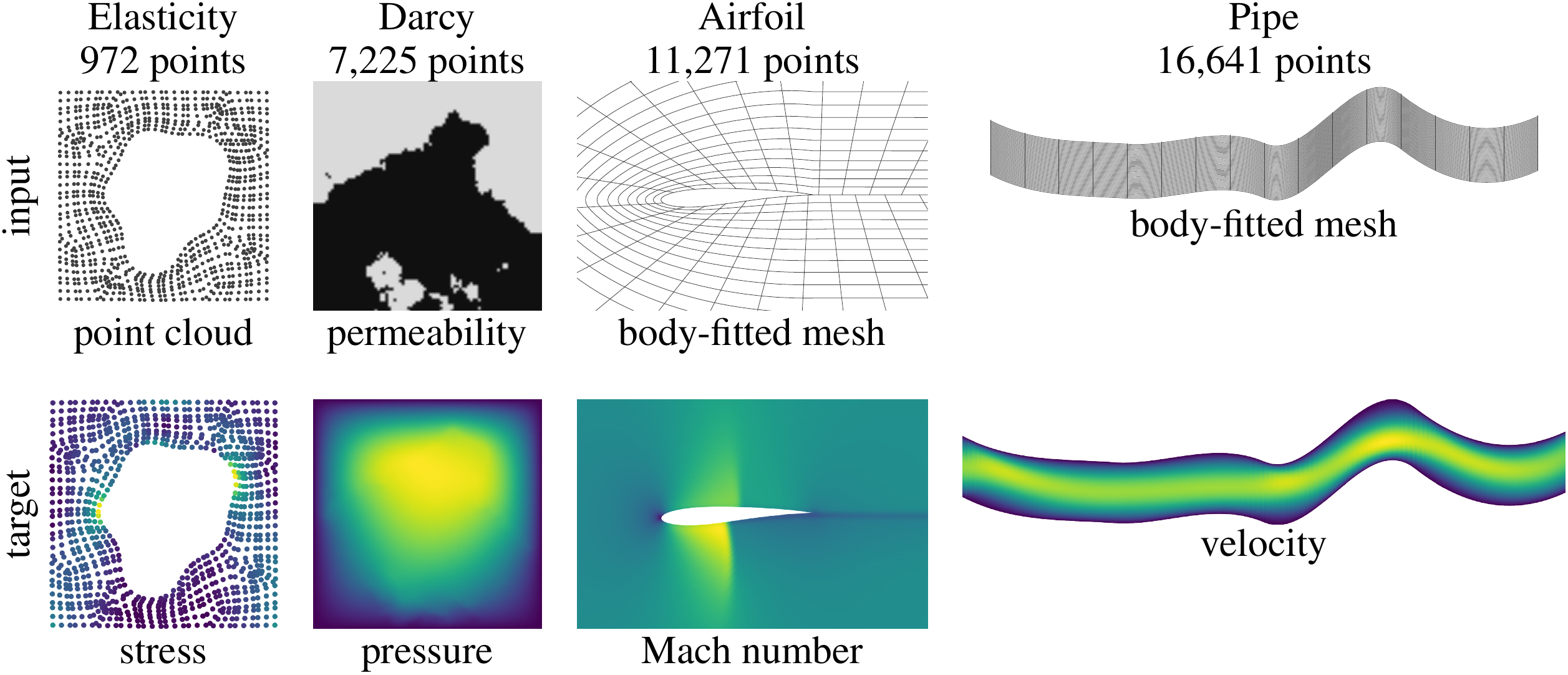
We compared token mixers inside a shared residual backbone: same width, heads, depth, latent budget, and training recipe per dataset, so the comparison isolates the mixer. Test relative $L^2$ error (%), FP32:
| Model | Elasticity | Darcy | Airfoil | Pipe | DrivAerML-40K |
|---|---|---|---|---|---|
| Full self-attention | 0.41 | 0.43 | 0.58 | – | – |
| Set Transformer | 0.57 | 1.18 | 0.67 | 0.39 | 6.56 |
| Luna | 0.59 | 0.84 | 0.60 | 0.38 | 6.90 |
| Transolver | 0.72 | 1.04 | 0.60 | 0.38 | 7.39 |
| Transolver-3 | 0.68 | 1.03 | 0.73 | 0.44 | 7.36 |
| AB-UPT | 1.34 | 2.70 | 2.93 | 4.12 | 10.0 |
| FLARE | 0.71 | 0.76 | 0.57 | 0.51 | 7.22 |
| FLARE++ | 0.39 | 0.62 | 0.50 | 0.35 | 5.80 |
Elasticity entries for FLARE and FLARE++ are means over ten seeds; full self-attention is omitted where it is prohibitively slow. The paper’s table also has PerceiverIO, GNOT, LNO, and Transolver++.
FLARE++ reduces FLARE’s error by 12–45% (25% on average) and has the lowest error among the efficient mixers on all five tasks. Full self-attention is the honest reference point: FLARE++ beats it on Elasticity and Airfoil, but full self-attention still has the lowest Darcy error.
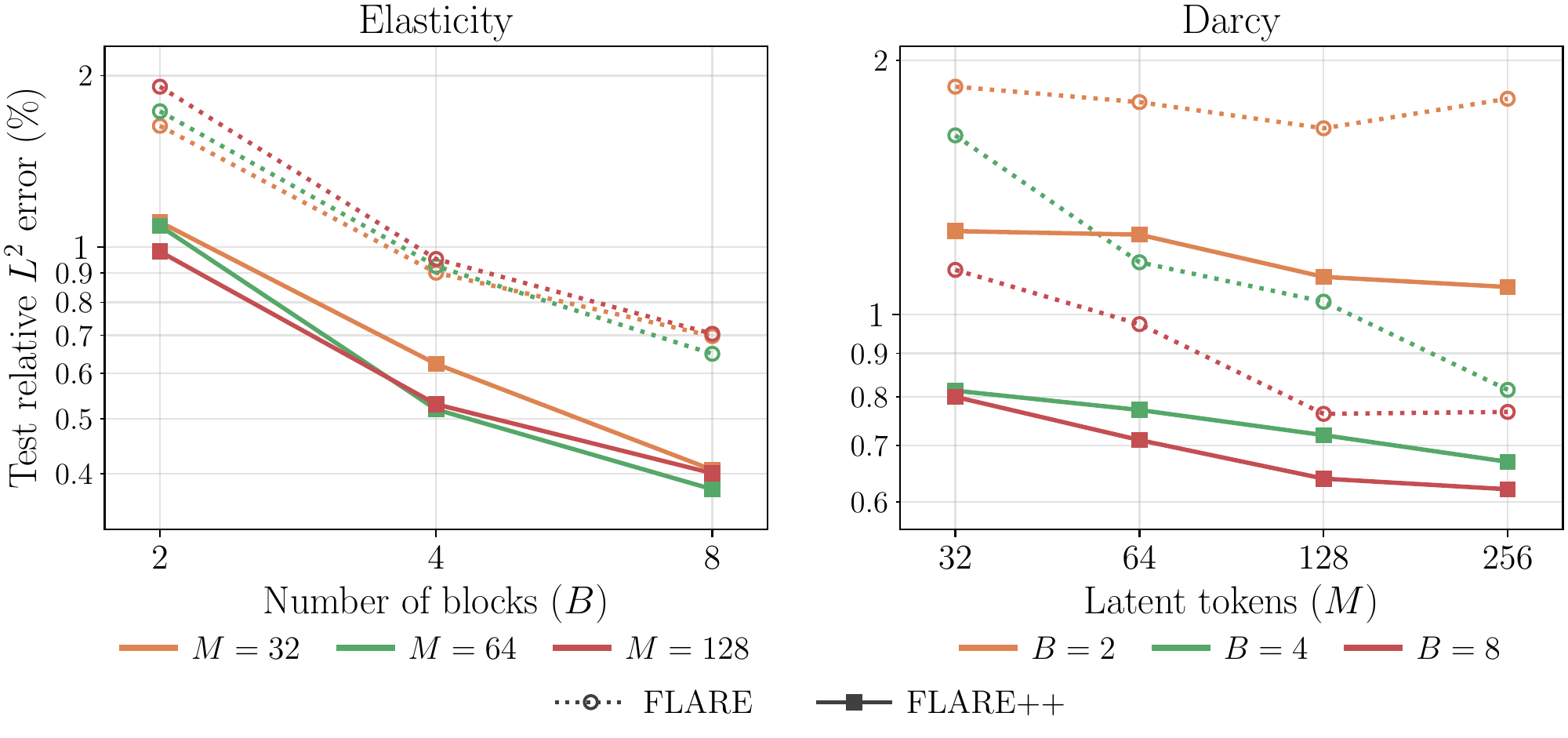
The gain is not something you get from a bigger latent budget or more depth. Across a joint sweep of latent budget $M$ and depth on Elasticity and Darcy, FLARE++ is more accurate in all 21 matched configurations, by 16–50%. On Elasticity, raising $M$ from 32 to 128 leaves FLARE flat while FLARE++ keeps improving, and at a fixed latent budget FLARE++ reaches a given error with a shallower model.
Full-surface DrivAerML
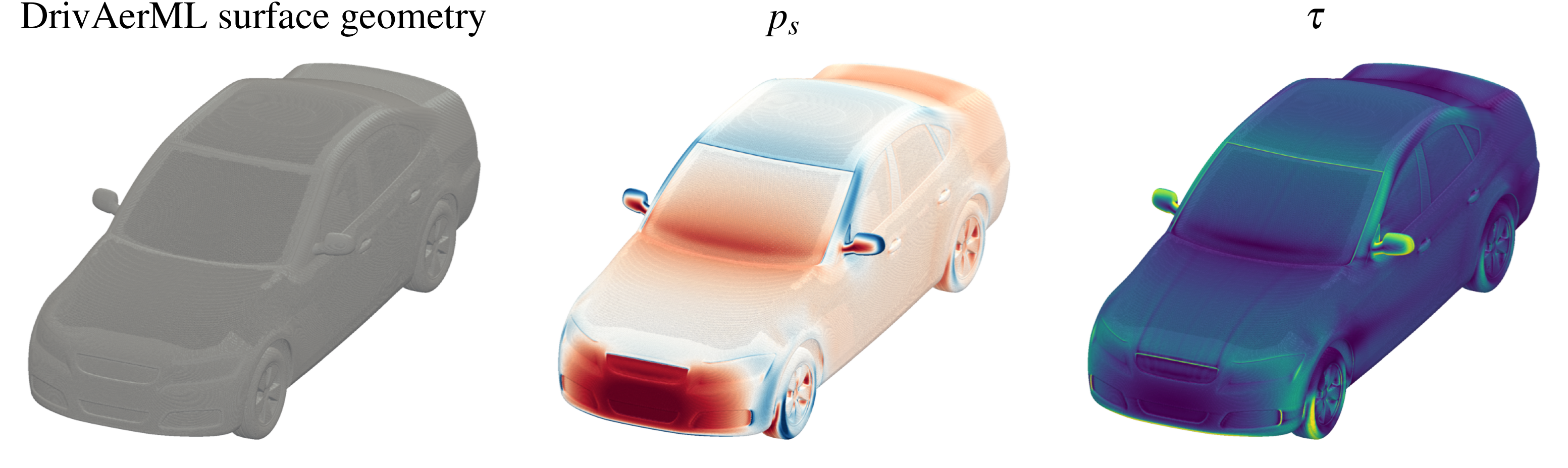
This is a different task from DrivAerML-40K above, so the numbers are not comparable. Here models predict surface pressure and three wall-shear components on the full 8.2M-cell car surface, trained on 100K sampled cells per step and evaluated on the entire surface in one pass using context parallelism.
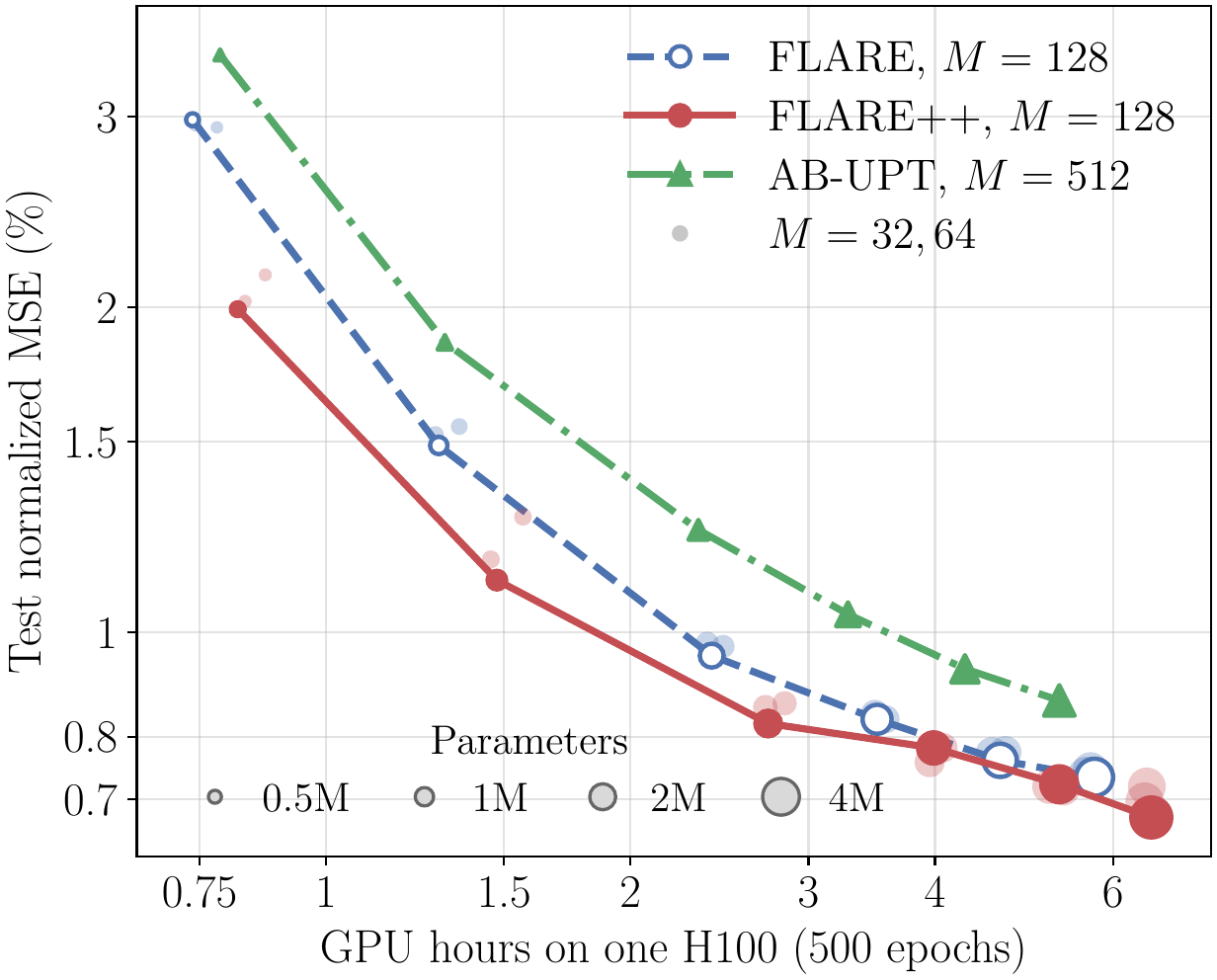
FLARE++ improves on FLARE in all 18 matched depth × latent-budget configurations: by 31% at two blocks, 22% at four, 13% at eight (averaged over latent budgets), shrinking to 6–7% in the deepest models. Plotted against training cost, a full FLARE++ run costs 1.1–1.2× the GPU hours of the matching FLARE run. Above about 3.4 GPU hours, every FLARE run is dominated by a FLARE++ run that is both cheaper and more accurate. Below 2.5 GPU hours the two alternate. AB-UPT, even with 512 anchors, has higher error than both at every depth.
Long Range Arena
To check the idea is not specific to physical fields, we dropped FLARE++ into FLARE’s LRA setup. It improves on FLARE on all five tasks, taking average accuracy from 58.08% to 61.60%, second to the published Luna result (61.95%).
What I take away from this
The rank-$M$ bottleneck is not only about how many routes you have but about where they point. With fixed queries, adding latents stopped helping on Elasticity; letting the input deform the queries kept the same budget useful. The cheapest place to get that input dependence turned out to be the operator we already had: FLARE’s encoder, called once more, with a gate to keep training well-behaved.
Open questions I am still thinking about: how far the gate actually moves from zero in trained models and what that says about when adaptivity matters, how the synthesized routes relate to geometry and topology on complex domains (the subject of a companion paper), and whether the same trick helps causal language modeling.
References
- Puri, V., Bandreddi, S. D. G., Zhang, Y. J., Kara, L. B. FLARE++: Low-rank attention with attention-synthesized routing. arXiv (2026). https://arxiv.org/abs/2608.11519
- Puri, V. et al. FLARE: Fast Low-rank Attention Routing Engine. arXiv (2025). https://arxiv.org/abs/2508.12594
- FLARE.py code repository. https://github.com/vpuri3/FLARE.py
- Jaegle, A. et al. Perceiver IO: A General Architecture for Structured Inputs & Outputs. ICLR (2022). https://arxiv.org/abs/2107.14795
- Wu, H. et al. Transolver: A Fast Transformer Solver for PDEs on General Geometries. ICML (2024). https://arxiv.org/abs/2402.02366
- Ma, X. et al. Luna: Linear Unified Nested Attention. NeurIPS (2021). https://arxiv.org/abs/2106.01540
- Alkin, B. et al. AB-UPT: Scaling Neural CFD Surrogates for High-Fidelity Automotive Aerodynamics Simulations via Anchored-Branched Universal Physics Transformers. (2025). https://arxiv.org/abs/2502.09692
- Liu, H. et al. Ring Attention with Blockwise Transformers for Near-Infinite Context. ICLR (2024). https://arxiv.org/abs/2310.01889
- Ashton, N. et al. DrivAerML: High-Fidelity Computational Fluid Dynamics Dataset for Road-Car External Aerodynamics. (2024). https://arxiv.org/abs/2408.11969
- Tay, Y. et al. Long Range Arena: A Benchmark for Efficient Transformers. ICLR (2021). https://arxiv.org/abs/2011.04006