Running notes — last updated 2026-03-02. This is a living document, not a polished article; I update it frequently as my understanding develops.
Motivation
FLARE was originally developed as an encoder-style global mixing primitive: learned latent queries gather information from many tokens, then scatter it back. The decoder setting is harder because causality changes algorithmic dependencies, numerical stability constraints, and what efficiency means in training versus inference.
This post summarizes a practical path to causal FLARE for long-context language modeling. See also the dissertation proposal talk for broader context.
What changes from encoder to decoder?
Encoder attention is bidirectional: token $t$ can depend on any token $\tau$. Decoder attention is causal: token $t$ may depend only on $\tau \le t$.
This implies three requirements:
- No future-token leakage.
- Efficient prefill for long contexts.
- Fast incremental decode with cached state.
Recap: encoder FLARE as gather-scatter
Let latent queries be $Q_L \in \mathbb{R}^{M \times D}$, and token keys/values be $K,V \in \mathbb{R}^{N \times D}$.
$$ Z = \mathrm{SDPA}(Q_L, K, V), \qquad Y = \mathrm{SDPA}(K, Q_L, Z). $$Interpretation:
- Gather: latents pool from tokens.
- Scatter: tokens read from latents.
Causal softmax attention baseline
$$ y_t = \sum_{\tau \le t} \frac{\exp(q_t^\top k_\tau)}{\sum_{u \le t}\exp(q_t^\top k_u)}v_\tau $$or
$$ Y = \mathrm{softmax}\!\big((QK^\top) \odot M_{\mathrm{causal}}\big)V, $$where $M_{\mathrm{causal}}$ masks the strict upper triangle.
Standard decoder attention therefore carries a variable-size state at inference time: the effective memory grows with the prefix because the model must retain the full KV cache for all prior tokens.
Warm-up: causal linear attention as a state update
$$ y_t = \frac{S_t q_t}{q_t^\top z_t}, \qquad S_t = \sum_{\tau \le t} v_\tau k_\tau^\top, \qquad z_t = \sum_{\tau \le t} k_\tau. $$This shows the decoder-friendly pattern: maintain prefix state, update incrementally, and compute $y_t$ from state plus $q_t$.
Causal FLARE definition
A causal latent update can be written as:
$$ z_m^t = \sum_{\tau \le t} \frac{\exp(q_m^\top k_\tau)}{\sum_{u \le t}\exp(q_m^\top k_u)}v_\tau. $$Then token output at step $t$:
$$ y_t = \sum_{m=1}^M \frac{\exp(k_t^\top q_m)}{\sum_{m'=1}^M \exp(k_t^\top q_{m'})} z_m^t. $$So each step produces an updated latent set $Z_t = [z_1^t,\ldots,z_M^t]$, then token $t$ reads from it.
Contrast with linear attention. Unnormalized linear attention accumulates $S_t = \sum_{\tau \le t} k_\tau v_\tau^\top$ without per-token normalization, forcing all queries to interact with the same global summary statistic. FLARE normalizes independently per latent, preserving query-specific weighting.
The key distinction from standard attention is the state shape: causal FLARE compresses the entire prefix into a fixed-size recurrent latent state $(\mu_t, d_t, U_t)$ with size $\mathcal{O}(M)$ per head, rather than a KV cache that grows with sequence length.
Contributions
- Causal FLARE formulation. Prefix-softmax normalization over $M$ latent queries admits an exact fixed-size recurrent state via the online-softmax algorithm: $\mathcal{O}(M)$ memory per head, no forgetting, and no approximation.
- Fixed-size state via prefix scan. Unlike standard causal attention, whose inference state grows with the prefix length through the KV cache, FLARE exposes a three-phase algorithm (chunk statistics → prefix scan → per-chunk recurrent decode) that preserves exactness while keeping the cached state size independent of context length.
- Triton GPU kernels. Fused Triton kernels for chunkwise prefill and recurrent decode eliminate PyTorch autograd overhead, minimize memory traffic, and deliver constant-time token generation with the fixed latent state.
- Empirical validation at 340M scale. Trained on 10B tokens of FineWeb, FLARE-LM matches GLA in training loss and downstream benchmarks (MMLU, CommonsenseQA, LongBench) while decode latency and memory remain constant with context length.
Algorithm 1: streaming recurrent causal FLARE (decode-friendly)
Each latent maintains running online-softmax statistics across the token stream: a running max $\mu_{t,m}$, a normalizing denominator $d_{t,m}$, and a numerator accumulator $U_{t,m,:}$. The update at each step is:
- Initialize:
- $U_0 \in \mathbb{R}^{M \times D} \leftarrow 0$
- $d_0 \in \mathbb{R}^{M} \leftarrow 0$
- $\mu_0 \in \mathbb{R}^{M} \leftarrow -\infty$
- For each token $t=1,\ldots,T$, given $(k_t, v_t)$:
- $s_t \leftarrow (Qk_t)s$
- $\mu_t \leftarrow \max(\mu_{t-1}, s_t)$
- $\gamma \leftarrow \exp(\mu_{t-1}-\mu_t)$
- $\eta \leftarrow \exp(s_t-\mu_t)$
- $d_t \leftarrow d_{t-1}\odot\gamma + \eta$
- $U_t \leftarrow U_{t-1}\odot\gamma + \eta\,v_t^\top$
- $Z_t \leftarrow U_t \oslash d_t$
- $\alpha_t \leftarrow \mathrm{softmax}(s_t)$
- $y_t \leftarrow \alpha_t^\top Z_t$
- Return $\{y_t\}_{t=1}^T$.
This recurrent form is ideal for autoregressive decode — cached state is updated in $O(M)$ work per token. However, it is throughput-inefficient for training because the backward pass must store all prefix statistics naively. The next two algorithms address the prefill and training setting.
import torch
import torch.nn.functional as F

def causal_flare_decode_step(q, k_t, v_t, U, d, mu, scale=1.0):
    """
    Algorithm 1: single recurrent step for autoregressive decode.

    Updates the cached latent state with the new token and reads the output.

    Args:
        q:   [H, M, D]     latent queries (learned, fixed across steps)
        k_t: [B, H, D]     key for the current token
        v_t: [B, H, D]     value for the current token
        U:   [B, H, M, D]  running numerator accumulator (fp32)
        d:   [B, H, M]     running denominator (fp32)
        mu:  [B, H, M]     running prefix max (fp32)
        scale: float       key-query scale factor (default 1.0)

    Returns:
        y_t: [B, H, D]     output for the current token
        U:   [B, H, M, D]  updated numerator accumulator
        d:   [B, H, M]     updated denominator
        mu:  [B, H, M]     updated prefix max
    """
    # s_t[b, h, m] = scale * dot(q[h, m], k_t[b, h])
    s_t = scale * torch.einsum('hmd,bhd->bhm', q, k_t.float())  # [B, H, M]

    # Online-softmax update for each latent
    mu_new  = torch.maximum(mu, s_t)                     # [B, H, M]
    gamma   = torch.exp(mu - mu_new)                     # rescale old stats
    eta     = torch.exp(s_t - mu_new)                    # weight for new token

    d  = d * gamma + eta                                 # [B, H, M]
    U  = U * gamma.unsqueeze(-1) + eta.unsqueeze(-1) * v_t.float().unsqueeze(2)  # [B, H, M, D]
    mu = mu_new

    Z_t = U / (d.unsqueeze(-1) + 1e-6)                  # [B, H, M, D]

    # Scatter: token reads from updated latents via softmax over M
    alpha_t = F.softmax(s_t, dim=-1)                     # [B, H, M]
    y_t = torch.einsum('bhm,bhmd->bhd', alpha_t, Z_t)   # [B, H, D]

    return y_t.to(v_t.dtype), U, d, mu
Why not a dense algorithm?
A natural question is whether causal FLARE admits a dense, matmul-friendly formulation that avoids the token loop entirely. Writing $S_{m\tau} = s\,q_m^\top k_\tau$ and $A_{m\tau} = \exp(S_{m\tau})$, the output can be expressed as
$$ y_t = \sum_{\tau \le t} W_{t\tau}\, v_\tau, \qquad W_{t\tau} = \sum_{m=1}^M \frac{P_{mt}}{D_{mt}} A_{m\tau}, $$where $P_{mt} = \mathrm{softmax}_m(S_{\cdot t})$ are the decode probabilities and $D_{mt} = \sum_{u \le t} A_{mu}$ is the prefix denominator. The full mixing matrix $W \in \mathbb{R}^{T \times T}$ can be written as $W = (P \oslash D)^\top \cdot A$, followed by a causal mask and matmul with $V$. This is a clean dense formulation.
The problem is numerical stability. Computing $D_{mt}$ requires the running prefix maximum
$$ R_{mt} = \max_{\tau \le t} S_{m\tau} $$for safe exponentiation. This maximum depends on the causal ordering and cannot be computed in a single parallel pass over $t$: a numerically stable version requires a sequential scan over $t$ to accumulate $R_{mt}$, which reintroduces a token loop and negates the benefit of the dense formulation.
The chunkwise algorithm below is the practical resolution: it amortizes the sequential dependency to a scan over chunks rather than individual tokens, exposing the parallelism that makes GPU kernels efficient.
Chunkwise forward algorithm (training / prefill)
The recurrent algorithm is ideal for decode but throughput-limited for training: the backward pass must store all prefix statistics for all $T$ steps. The practical resolution is to amortize the sequential dependency to a scan over chunks rather than individual tokens.
Fix a chunk length $C$ and define $N = T/C$ chunks with index sets $I_c = \{(c-1)C+1,\ldots,cC\}$.
Phase 1 — chunk-local statistics (parallel over chunks). For each chunk $c$, compute independently:
$$ \mu^{(c)} = \max_{t \in I_c}(s\,Qk_t^\top), \quad d^{(c)} = \sum_{t \in I_c} \exp(s\,Qk_t^\top - \mu^{(c)}), \quad U^{(c)} = \sum_{t \in I_c} \exp(s\,Qk_t^\top - \mu^{(c)})\,v_t^\top. $$This is fully parallel over $N$ chunks.
Phase 2 — prefix scan over chunks (sequential over $N$ chunks). Combine chunk summaries with online-softmax merging:
$$ \tilde\mu^{(c)} = \max(\tilde\mu^{(c-1)}, \mu^{(c)}), \quad \gamma^{(c)} = \exp(\tilde\mu^{(c-1)} - \tilde\mu^{(c)}), \quad \eta^{(c)} = \exp(\mu^{(c)} - \tilde\mu^{(c)}), $$$$ \tilde{d}^{(c)} = \tilde{d}^{(c-1)} \odot \gamma^{(c)} + d^{(c)} \odot \eta^{(c)}, \quad \tilde{U}^{(c)} = \tilde{U}^{(c-1)} \odot \gamma^{(c)} + U^{(c)} \odot \eta^{(c)}. $$The exclusive prefix state for chunk $c$ is $(\tilde\mu^{(c-1)}, \tilde{d}^{(c-1)}, \tilde{U}^{(c-1)})$.
Phase 3 — recurrent decode within each chunk (parallel over chunks). Initialize each chunk’s recurrent pass at its exclusive prefix state and run Algorithm 1 over the $C$ tokens of that chunk. Since the prefix scan has already accounted for all earlier tokens, each chunk produces the same outputs as a fully sequential pass — and all chunks run in parallel.
The sequential work is now $\mathcal{O}(N) = \mathcal{O}(T/C)$ rather than $\mathcal{O}(T)$. For $C = 64$ this is a $64\times$ reduction in the sequential bottleneck, and $N$ is small enough that the Phase 2 scan is negligible on modern GPUs.
Algorithm 2: Chunkwise FLARE Forward Pass (training / prefill)

Input:  Q ∈ R^{M×D}, keys {k_t}, values {v_t} for t=1..T,
        scale s, chunk length C  (assume T = NC)
Output: {y_t} for t=1..T

Define chunk index sets I_c = {(c-1)C+1, ..., cC} for c = 1..N

── Phase 1: chunk-local statistics (parallel over all chunks) ──────────
for each chunk c in parallel:
    μ^(c)  ← max_{t ∈ I_c}  s·Q k_t^T          ∈ R^M
    d^(c)  ← Σ_{t ∈ I_c}   exp(s·Qk_t^T − μ^(c))     ∈ R^M
    U^(c)  ← Σ_{t ∈ I_c}   exp(s·Qk_t^T − μ^(c)) · v_t^T  ∈ R^{M×D}

── Phase 2: prefix scan over chunks (sequential over c = 1..N) ─────────
init: μ̃^(0) ← −∞,  d̃^(0) ← 0,  Ũ^(0) ← 0
for c = 1..N:
    μ̃^(c) ← max(μ̃^(c−1), μ^(c))
    γ^(c)  ← exp(μ̃^(c−1) − μ̃^(c))
    η^(c)  ← exp(μ^(c)    − μ̃^(c))
    d̃^(c) ← d̃^(c−1) ⊙ γ^(c) + d^(c) ⊙ η^(c)
    Ũ^(c) ← Ũ^(c−1) ⊙ γ^(c) + U^(c) ⊙ η^(c)

exclusive prefix init for chunk c:
    (μ_0^(c), d_0^(c), U_0^(c)) ← (μ̃^(c−1), d̃^(c−1), Ũ^(c−1))

── Phase 3: recurrent decode within each chunk (parallel over all chunks)
for each chunk c in parallel:
    run Algorithm 1 on {k_t, v_t}_{t ∈ I_c}
    initialized at (μ_0^(c), d_0^(c), U_0^(c))

return {y_t}
Train vs prefill vs decode
Causal FLARE supports three operational regimes, each with different priorities.
Training is throughput-oriented and uses chunkwise processing. Algorithm 1 is the inner hot-loop kernel for each chunk ($C \approx 32$–$128$): its recurrent token pass fits in registers and achieves high occupancy. The inter-chunk prefix denominator $D_{\text{prefix},m}$ is accumulated between chunks via a running sum. Algorithm 3 is the right choice when a larger-chunk or full-sequence dense kernel is preferred and the sequential prefix-statistics pass is acceptable.
Inference prefill is algorithmically identical to training but with a different blocking profile. Prefill is latency-sensitive and may benefit from different tile sizes and more aggressive kernel fusion than the training path.
Autoregressive decode is latency-critical and processes one token at a time. Algorithm 1 is ideal: update the cached latent state with each new $(k_t, v_t)$, then read $y_t$ from the updated latents. No attention matrix is ever constructed, and the state size $M$ is the only memory overhead beyond the KV cache.
Results
All models have ~340M parameters (24 blocks, hidden dim 1024, 16 heads) and are trained on 10B tokens of FineWeb with sequence length 2048.
Training loss
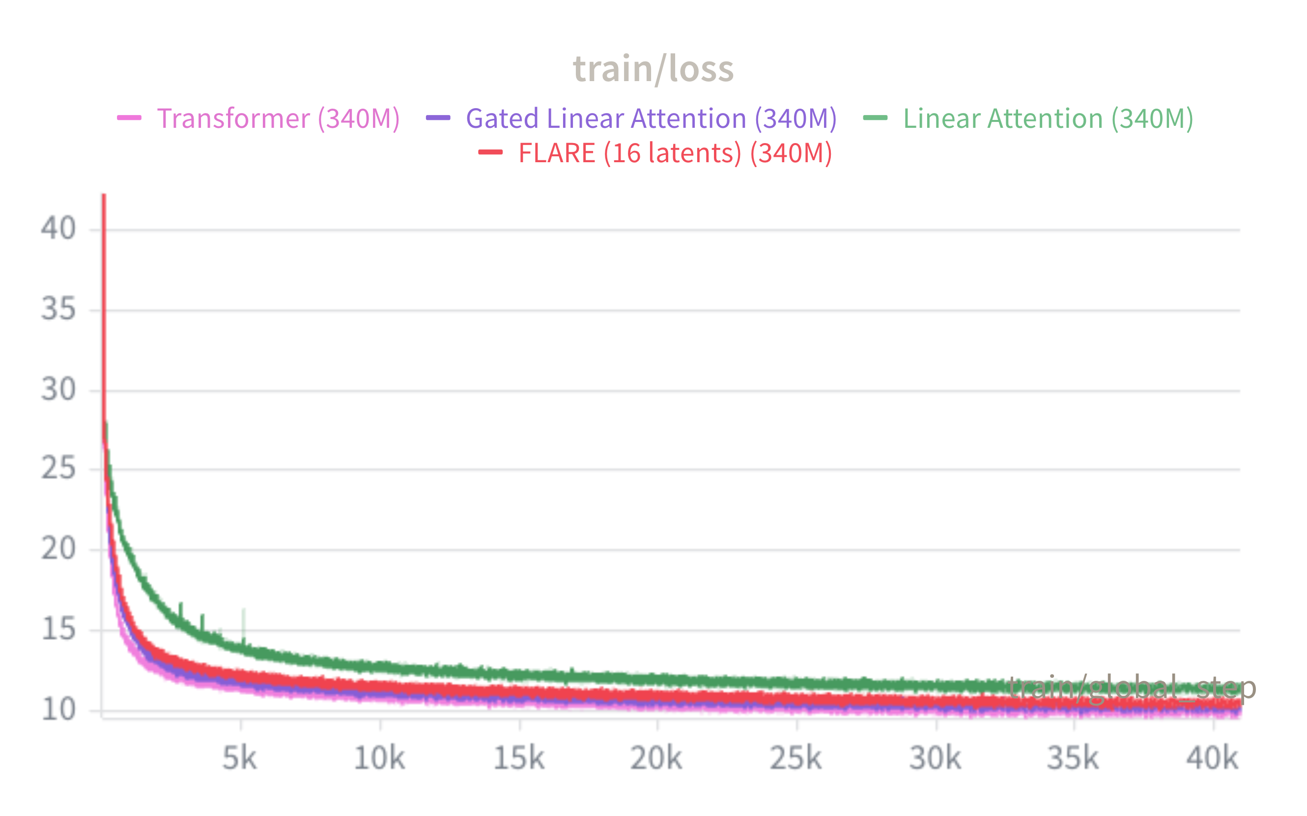
FLARE (16 latents, red) closely tracks Transformer++ throughout training and is competitive with GLA, while unmodified Linear Attention converges to a noticeably higher loss. This confirms that prefix normalization — without any forgetting — is a strong inductive bias: routing through only $M=16$ latent queries per head largely recovers the expressive power of full softmax attention.
Downstream benchmarks
| Model | Params | Train loss↓ | MMLU↑ | CSR↑ | Lambada↑ | Wiki PPL↓ | LongBench↑ |
|---|---|---|---|---|---|---|---|
| Linear Attention | 316M | 11.38 | 0.256 | 0.447 | 0.195 | 48.04 | N/A |
| GLA | 342M | 10.23 | 0.267 | 0.470 | 0.312 | 31.85 | 0.082 |
| Transformer++ | 341M | 9.93 | 0.253 | 0.473 | 0.347 | 28.06 | 0.078 |
| FLARE-LM ($M=16$) | 316M | 10.50 | 0.244 | 0.466 | 0.243 | 35.04 | 0.064 |
FLARE is competitive with GLA across MMLU and CommonsenseQA; both sublinear-memory methods trail Transformer++ modestly on perplexity and Lambada.
Prefill and decode throughput
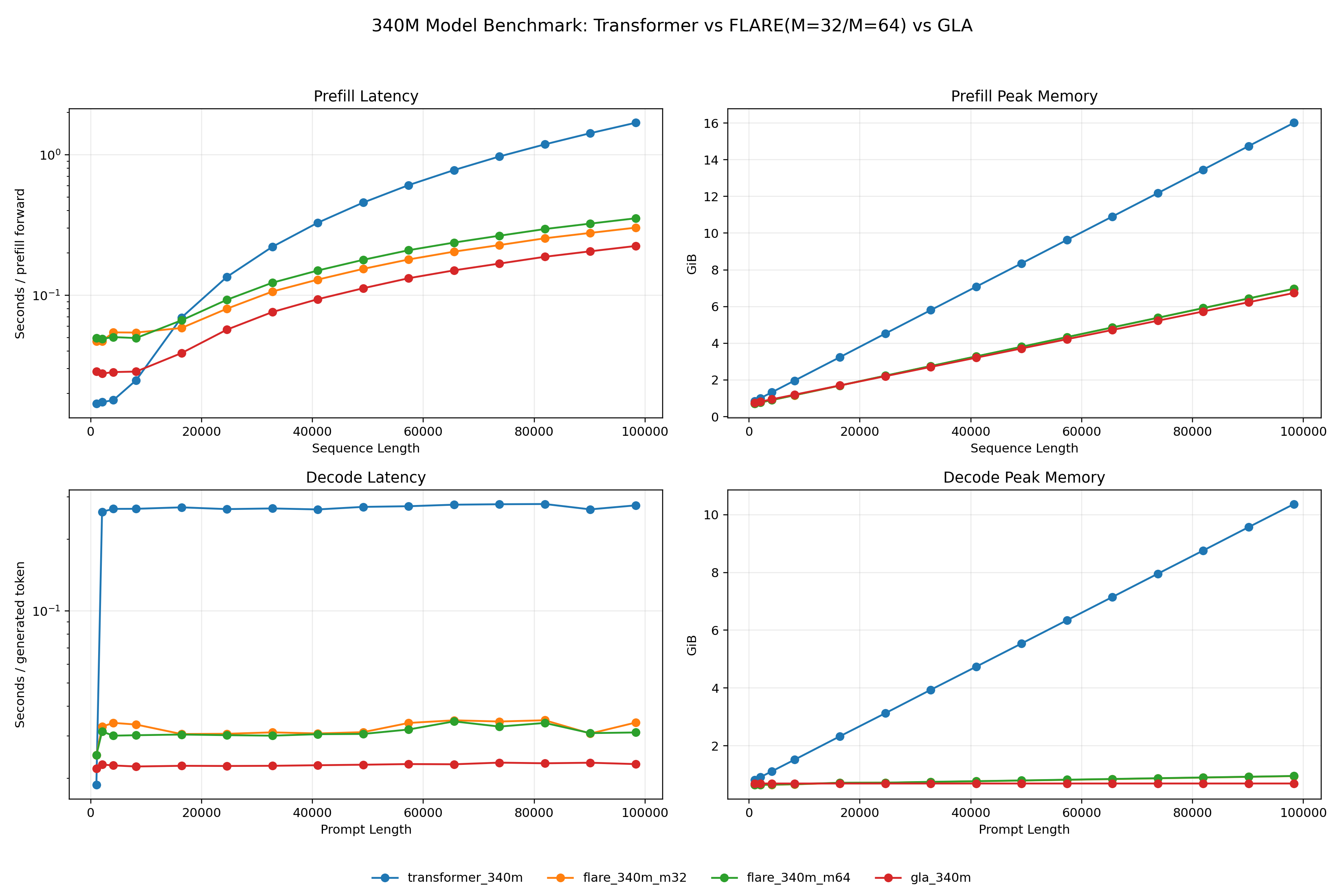
For prefill (top row), FLARE’s chunkwise kernel achieves substantially lower latency and peak memory than Transformer, whose quadratic attention dominates at long sequences. Decode (bottom row) is the clearer differentiator: Transformer latency and memory grow linearly with prompt length due to the KV-cache, while FLARE’s recurrent state is fixed at $\mathcal{O}(MD)$ regardless. At 100k tokens, FLARE ($M=32$) uses roughly $10\times$ less decode memory than Transformer, with flat latency across all prompt lengths.
Adaptive attention state size
- More states mean more latency? Can we adaptively drop latents at inference time?
- Think of latent tokens as experts in MoE? Can we add more latents at finetune time to learn new capabilities?
This exposes a direct compute vs. accuracy tradeoff.
Systems notes
A few implementation details matter disproportionately.
FP32 prefix accumulators. The running max and sum statistics accumulate error across many tokens. Accumulating in FP32 prevents catastrophic cancellation even when inputs are in BF16 or FP16.
Time chunking. Processing time in chunks avoids materializing the full $T \times T$ intermediate — which is precisely the goal. Chunk size trades register pressure against memory traffic and should be tuned per GPU.
Separate kernels per regime. Training, prefill, and decode have different access patterns and arithmetic intensities. A single fused kernel cannot be optimally tiled for all three; separate kernels let you autotune each independently.
Memory bandwidth first. At long contexts, causal FLARE is memory-bandwidth-bound rather than compute-bound. Optimizing cache layout and minimizing global memory traffic matters more than maximizing FLOPs/s.
Future directions
Scaling to 1.3B / 100B tokens. The 340M / 10B run establishes a proof of concept. The standard evaluation configuration for SSM and linear attention baselines (Mamba, GLA, RetNet) is 1.3B parameters trained on 100B tokens — the setting needed to make direct comparisons. A secondary question is how the optimal $M$ scales with model size.
Long-context training. Current training uses sequences of length 2048. The memory advantage of FLARE only fully materializes at longer contexts, motivating training at 8k–32k tokens. The key enabler is a FlashAttention-2-style fused backward kernel: saving only the per-token log-normalizer $\ell_t \in \mathbb{R}^M$ and recomputing $Z_t$ on the fly reduces activation memory from $\mathcal{O}(MT)$ to $\mathcal{O}(M)$, making long-sequence training feasible without gradient checkpointing overhead. With long-context pretraining in place, evaluation targets include RULER, SCROLLS, and $\infty$Bench.
Architecture exploration. Three axes:
- Forgetting gates. A per-latent decay $\lambda_m \in (0,1]$ interpolates between full-prefix memory and aggressive forgetting, connecting FLARE-LM to Mamba and GLA while retaining prefix normalization.
- Hybrid models. Alternating FLARE layers with sliding-window local attention handles both global context (FLARE, $\mathcal{O}(NM)$) and fine-grained local dependencies.
- Content-aware latent queries. Making $Q$ prefix-dependent enables dynamic routing, potentially improving expressivity on code and mathematics.
Inference-time deployment. At 100k+ tokens, FLARE’s fixed $\mathcal{O}(M \times D)$ state is the main differentiator against quantized KV-cache and sliding-window baselines. The recurrent state $(\mu_t, d_t, U_t)$ also enables prompt caching: serialize the prefix state once, reuse across requests in multi-turn and agent settings.
References
- Puri, V. et al. FLARE: Fast Low-rank Attention Routing Engine. arXiv (2025). https://arxiv.org/abs/2508.12594
- Vaswani, A. et al. Attention Is All You Need. NeurIPS (2017). https://arxiv.org/abs/1706.03762
- Dao, T. et al. FlashAttention: Fast and Memory-Efficient Exact Attention with IO-Awareness. NeurIPS (2022). https://arxiv.org/abs/2205.14135
- Qin, Z. et al. The Devil in Linear Transformer. arXiv (2022). https://arxiv.org/abs/2210.10340
- FLARE.py.
lra/models/triton/causal_linear.py. https://github.com/vpuri3/FLARE.py/blob/master/lra/models/triton/causal_linear.py - Gu, A. and Dao, T. Mamba: Linear-Time Sequence Modeling with Selective State Spaces. arXiv (2023). https://arxiv.org/abs/2312.00752
- Yang, S. et al. Gated Linear Attention Transformers with Hardware-Efficient Training. arXiv (2024). https://arxiv.org/abs/2312.06635
- Penedo, G. et al. The FineWeb Datasets: Decanting the Web for the Finest Text Data at Scale. NeurIPS (2024). https://huggingface.co/datasets/HuggingFaceFW/fineweb
- Hsieh, C.-P. et al. RULER: What’s the Real Context Window Size of Your Long-Context Language Models? arXiv (2024). https://arxiv.org/abs/2404.06654