From POD to neural manifolds: a modern take on reduced order modeling

From POD to neural manifolds

Reduced-order modeling (ROM) is ultimately about preserving dominant system behavior with far fewer degrees of freedom. Classical projection methods, convolutional autoencoder ROMs, and modern neural-field formulations all target this same objective, but they make different assumptions about (i) how we represent the state and (ii) how we evolve it in time.

This post walks through that progression and focuses on Smooth Neural Field ROM (SNF-ROM): a projection-based nonlinear ROM that uses continuous neural fields as the state representation and explicitly supports physics-based differentiation and time integration during deployment.

Preprint: arXiv:2405.14890

J. Comp. Phys. paper: https://doi.org/10.1016/j.jcp.2025.113957

See my dissertation proposal talk on this topic!

Why ROM matters for engineering workflows

High-fidelity simulation is now central to modern engineering pipelines, from fluid mechanics to control and design. However, high accuracy typically requires resolving many spatial and temporal scales, which makes PDE solves expensive. These costs become the bottleneck in workflows that require repeated evaluations, such as design-space exploration, optimization, and uncertainty quantification.

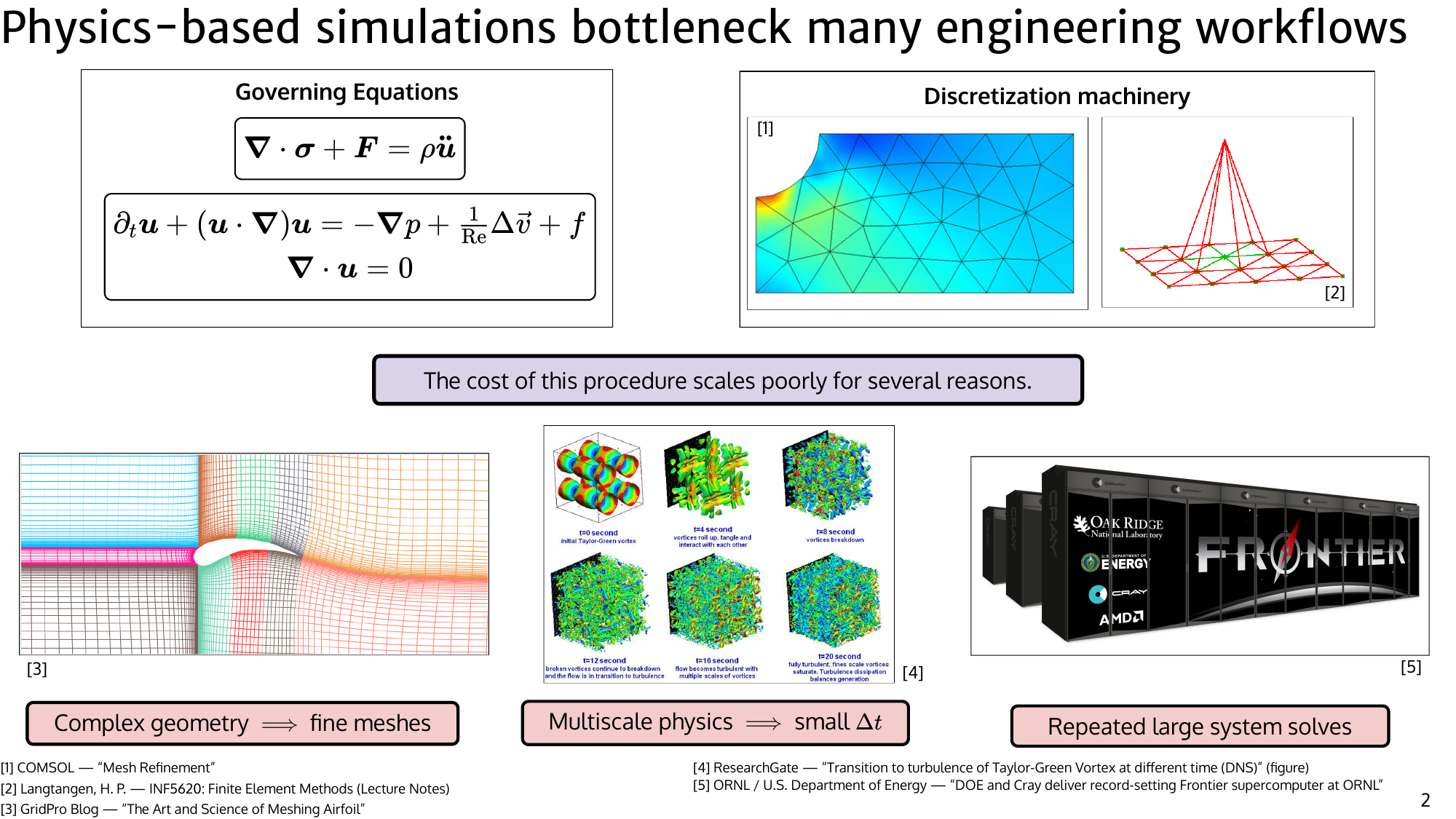
Machine learning offers a complementary approach to accelerating simulation. Instead of solving the full PDE from scratch every time, we can learn a surrogate model from data generated by high-fidelity simulations. Training such models can be computationally expensive, since they must observe many examples across parameter settings, geometries, and time horizons. But this cost is paid once offline. At deployment time, the learned model can evaluate new scenarios orders of magnitude faster than a traditional solver, making it attractive for design optimization, uncertainty quantification, control, and real-time decision-making workflows. In this sense, machine learning amortizes the cost of expensive PDE solves across many downstream queries.

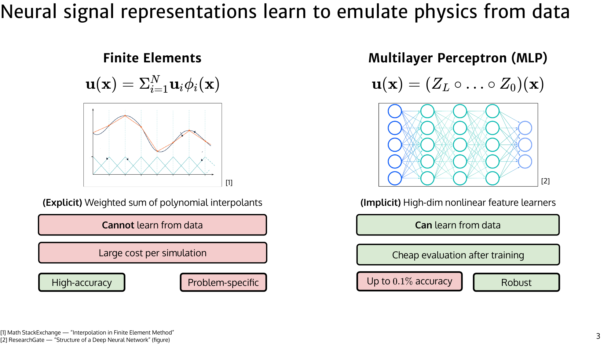
A particularly important class of surrogates is reduced-order models (ROMs). The central idea behind ROMs is that although PDE states live in extremely high-dimensional spaces (millions of degrees of freedom in realistic simulations), the effective dynamics often evolve on a much lower-dimensional structure. ROMs aim to discover this structure and use it to simulate the system using far fewer variables. Traditionally, this was done with linear subspace methods such as Proper Orthogonal Decomposition (POD) combined with Galerkin projection. Modern approaches extend this idea using machine learning to learn nonlinear representations that can better capture complex dynamics.

In this post, we focus on neural reduced-order modeling: learn a low-dimensional representation directly from data, then evolve that representation using physics-aware structure. Instead of predicting the full state everywhere, the model predicts a compact latent state that encodes the dominant behavior of the system, and the full field can be reconstructed from this latent representation. This separates the problem into two parts: representing the state efficiently and modeling how that representation evolves in time.

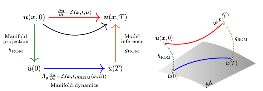
Before diving into SNF-ROM, it is helpful to recall the manifold learning viewpoint that underlies most nonlinear ROM methods. The core assumption is that although simulation states are extremely high-dimensional, they often lie close to a smooth, low-dimensional manifold embedded in the ambient space. For example, fluid flow snapshots over time may evolve primarily along a small number of coherent structures or modes. Learning this manifold provides a natural coordinate system in which the dynamics can be expressed compactly, and the role of a ROM is to learn both the geometry of this manifold and the dynamics that govern motion along it.

This perspective is illustrated by contrasting the full-order model (FOM) with linear and nonlinear ROMs. The governing PDE can be written abstractly as

$$ \frac{\partial u}{\partial t} = \mathcal{L}(x,t,u;\mu), $$

where $u(x,t;\mu)$ is the high-dimensional state, $x$ is spatial position, $t$ is time, and $\mu$ denotes parameters. In a full discretization, the state is represented as

$$ u(x,t;\mu) \approx g_{\mathrm{FOM}}(x,\bar u(t;\mu)) = \Phi(x),\bar u(t;\mu), $$

where $\Phi(x)$ is a spatial basis and $\bar u \in \mathbb{R}^{N_{\mathrm{FOM}}}$ are high-dimensional coefficients. A linear POD-ROM assumes the dynamics evolve in a low-dimensional linear subspace,

$$ \bar u(t;\mu) \approx \bar u_0 + \mathbf{P},\tilde u(t;\mu), $$

where $\mathbf{P}$ is a projection matrix and $\tilde u \in \mathbb{R}^{N_{\mathrm{Lin\text{-}ROM}}}$ are reduced coordinates. A nonlinear ROM instead assumes the state lies on a curved manifold and uses a learned decoder,

$$ u(x,t;\mu) \approx g_{\mathrm{ROM}}(x,\tilde u(t;\mu)) = \mathrm{NN}_\theta(x,\tilde u(t;\mu)), $$

where $\mathrm{NN}_\theta$ is a neural field mapping spatial coordinates and latent variables to the state. The dimensionality relationship

$$ N_{\mathrm{NI\text{-}ROM}} \le N_{\mathrm{Lin\text{-}ROM}} \ll N_{\mathrm{FOM}} $$

captures the intuition that nonlinear manifolds can often represent system behavior with fewer degrees of freedom than linear subspaces while still approximating the full system accurately.

Limitations of current ROMs (why nonlinear + why “smooth”)

It’s tempting to think ROM is “solved” once you can compress snapshots well. The hard part is what happens online, when you traverse the reduced manifold according to the governing PDE.

1) Linear subspace ROMs can be fundamentally inefficient

Classical POD-ROM assumes solutions live near a linear subspace. This works best when the Kolmogorov $n$-width decays quickly (roughly: a small number of modes captures most variation). But in advection-dominated flows and other problems with slow Kolmogorov $n$-width decay, the number of POD modes required for accuracy can become large, reducing speedups and sometimes harming stability.

2) Nonlinear ROMs often struggle where physics enters: derivatives

Neural manifold ROMs (e.g., CAE-ROM) can achieve excellent compression, but online physics requires evaluating spatial operators: gradients, Laplacians, Jacobians of the decoder map, and so on. A recurring practical issue is that neural fields are not guaranteed to interpolate smoothly, and their spatial derivatives can be noisy. If your derivative estimates are wrong, your dynamics are wrong.

Many nonlinear ROM pipelines handle this by introducing a coarse auxiliary grid and applying low-order finite differences for derivatives. That workaround can:

• require maintaining a background mesh (extra memory and engineering),
• introduce sensitivity to differencing hyperparameters,
• become brittle near boundaries, shocks, or sharp features.

The punchline is: if you want to do physics-based online integration, you need reliable differentiation through your representation.

SNF-ROM is designed around this constraint.

Where convolutional autoencoder ROMs struggle

Convolutional autoencoder ROMs can compress state fields effectively, but the compression/decompression workflow does not directly control latent trajectory quality during online integration. In practice, this mismatch can produce drift and degraded physical consistency.

There are two coupled issues:

1. The learned manifold may be accurate at training snapshots but poorly behaved between them.
2. The decoder’s derivatives (needed for dynamics) can be inaccurate or unstable.

If the online stage uses the PDE to evolve the reduced state, small derivative errors can compound quickly.

SNF-ROM: physics-based dynamics with neural fields

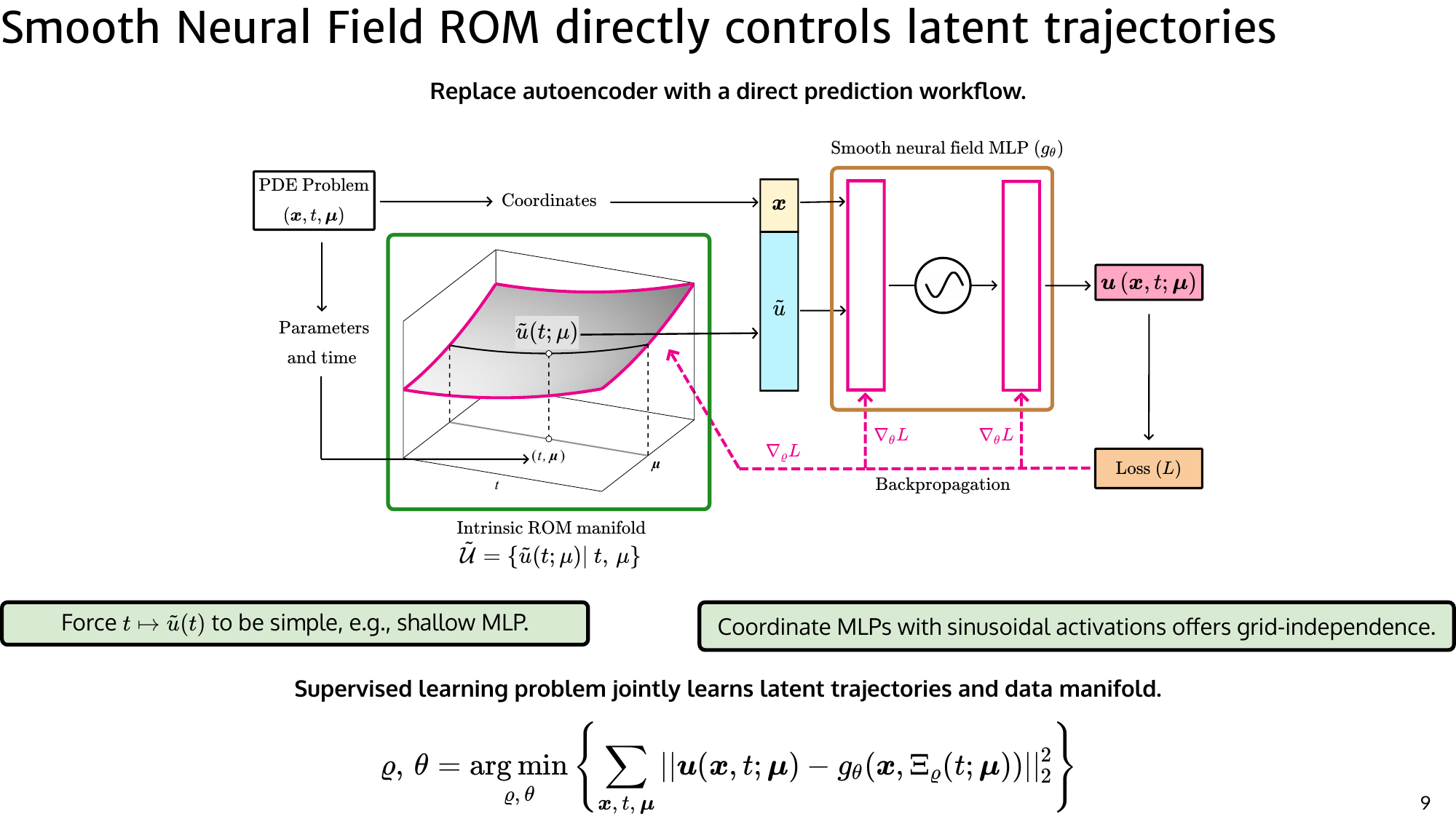
SNF-ROM is a projection-based nonlinear ROM that aims to keep the best parts of classical ROMs — Galerkin projection and classical time integrators — while replacing linear subspaces with a modern, continuous neural field representation. The key idea is not just to compress the state, but to build a representation on which the governing physics can be evaluated reliably during deployment.

Two design choices are central.

1. Constrained manifold formulation (trajectory regularity)

In classical ROMs, the reduced state evolves in a low-dimensional coordinate system whose geometry is fixed by the chosen basis. In nonlinear ROMs, this coordinate system becomes a learned manifold. However, if this manifold is irregular or poorly behaved between training samples, trajectories computed during online integration can drift or become numerically unstable.

SNF-ROM addresses this by explicitly modeling the reduced state as a smooth function of parameters and time. Conceptually, instead of learning isolated latent codes for snapshots, the model learns a continuous mapping

$$ \tilde{u} = \tilde{u}(t, \mu), $$

where $\tilde{u} \in \mathbb{R}^r$ is the reduced state. This encourages trajectories that vary smoothly as time evolves or parameters change. From a numerical perspective, this matters because online deployment involves stepping along this manifold using the governing PDE. If the manifold has sharp curvature or local irregularities, small integration errors can amplify. Enforcing trajectory regularity therefore improves stability and allows larger time steps during reduced-order integration.

2. Neural field regularization (derivative fidelity)

The second design choice focuses on the representation of the physical state itself. SNF-ROM uses a neural field decoder

$$ u(x,t;\mu) \approx f_\theta(x, \tilde{u}(t,\mu)), $$

which maps spatial coordinates and reduced variables to field values. Because the governing PDE involves spatial operators (gradients, Laplacians, fluxes), the accuracy of these derivatives is critical. Standard neural decoders can produce visually accurate reconstructions while still having noisy or oscillatory derivatives, which leads to incorrect physics when evaluating operators.

SNF-ROM therefore explicitly regularizes the neural field to encourage smoothness and suppress high-frequency artifacts. This improves derivative fidelity so that operators like

$$ \nabla u, \quad \Delta u, \quad \mathcal{L}(u) $$

can be computed using automatic differentiation. The key benefit is that PDE operators are evaluated directly on the learned representation without relying on auxiliary grids or finite-difference approximations. This makes the reduced model both grid-free and numerically stable.

Together, these two components are aimed at one goal: do physics on the learned manifold, not just reconstruction. The model is trained so that both the geometry of the manifold and the operators acting on it are well behaved during online simulation.

A key technical point is differentiability quality. If derivatives of the learned field are noisy, PDE-consistent inference degrades because the projected dynamics depend directly on these derivatives. By enforcing smooth neural fields, SNF-ROM ensures that gradients and higher-order operators remain accurate and stable during integration.

What SNF-ROM is doing (high level)

SNF-ROM uses a neural field decoder that maps coordinates and a low-dimensional latent to a field value:

• Neural field (continuous decoder):
  $$u(\mathbf{x}, t; \boldsymbol{\mu}) \approx f_\theta(\mathbf{x}, \tilde{u}(t,\boldsymbol{\mu}))$$

• Reduced state: $\tilde{u}(t,\boldsymbol{\mu}) \in \mathbb{R}^r$ is the low-dimensional ROM state.

During the online stage, SNF-ROM evolves $\tilde{u}(t)$ using projection-based dynamics, while evaluating the PDE operators through AD on the neural field. This is the “physics with neural fields” part: you can differentiate the representation to form operators needed for the reduced dynamics, and then integrate the resulting reduced ODE with standard time-stepping.

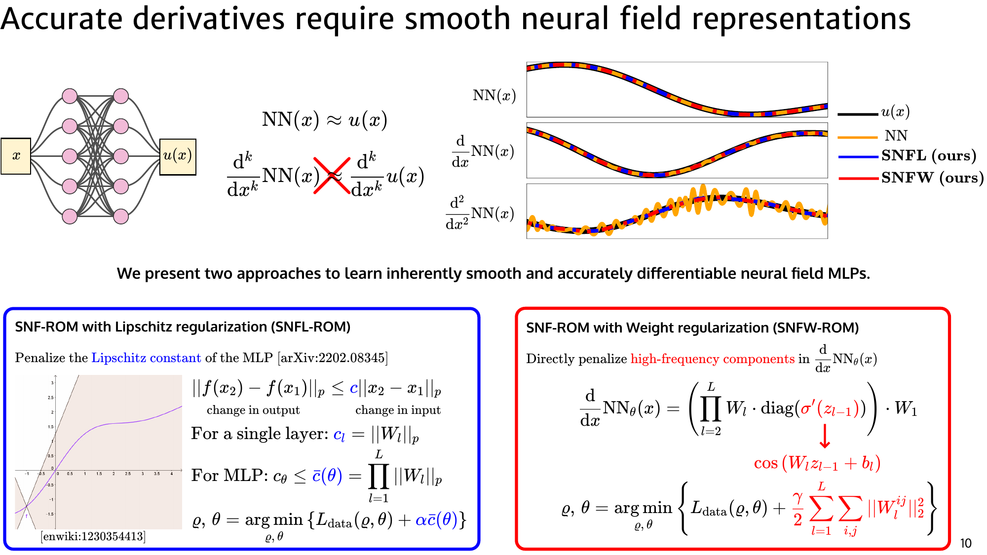
Smoothness: two regularized variants

The paper presents two regularized variants designed to suppress high-frequency artifacts in derivatives:

• SNFL-ROM: Lipschitz-style regularization to encourage smooth neural mappings.
• SNFW-ROM: weight regularization motivated by controlling oscillations that appear in derivative expressions (particularly relevant with sinusoidal activations).

Both are designed to produce smooth neural fields whose derivatives match the underlying signal more closely, which improves robustness during deployment-time dynamics evaluation.

Results

1D viscous Burgers

SNF-ROM variants maintain latent trajectory agreement under online solves where baseline CAE-ROM trajectories deviate.

1D Kuramoto–Sivashinsky

SNF-ROM maintains low relative error, including at larger time steps where baselines degrade.

2D viscous Burgers

The method achieves strong accuracy–speed tradeoffs with substantial state-space compression and high practical speed-up.

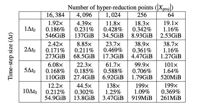
Speedup via hyper-reduction

A major practical benefit of SNF-ROM is the ability to dramatically reduce the cost of evaluating the governing equations through hyper-reduction. In a full-order model, evaluating the PDE residual requires computing operators over every spatial degree of freedom. For large simulations, this can involve hundreds of thousands or millions of points.

In SNF-ROM, the state is represented in a low-dimensional latent space, and projection allows the governing dynamics to be evaluated in this reduced coordinate system. Hyper-reduction further accelerates computation by evaluating nonlinear operators at a carefully selected subset of spatial locations rather than the full grid, while still preserving accuracy in the projected dynamics.

This combination leads to substantial speedups. In the reported experiment, a problem with roughly 500,000 spatial degrees of freedom is reduced to a latent system with just two variables, and the resulting reduced model achieves approximately 199× speedup compared to evaluating the full-order model. The key insight is that once the dominant dynamics are captured in a low-dimensional manifold, the cost of simulation is governed by the reduced dimension rather than the original spatial resolution, enabling large performance gains while maintaining accuracy.

Core contributions (what to remember)

SNF-ROM is best understood as a ROM framework that explicitly supports doing physics on a learned nonlinear manifold:

1. A constrained manifold formulation that encourages smoothly varying reduced trajectories, which improves online stability and allows larger time steps in practice.
2. Smooth neural field regularization that makes the representation reliably differentiable, enabling accurate spatial derivatives via automatic differentiation.
3. Nonintrusive, grid-free dynamics evaluation that works directly with point-cloud data, avoiding auxiliary meshes and brittle finite-difference derivative hacks.
4. Projection + classical integration: dynamics are evaluated in a physics-consistent way and integrated using standard time integrators, rather than relying purely on black-box latent dynamics predictors.

Takeaways

1. ROM quality depends not just on compression, but on controllable and stable online dynamics.
2. If your ROM uses the PDE online, derivative fidelity is not optional. Smoothness of the representation matters.
3. SNF-ROM shows that regularizing neural manifolds for differentiation + integration can materially improve robustness over standard autoencoder-based ROM pipelines.

References

- Puri, V. et al. SNF-ROM: Projection-based nonlinear reduced order modeling with smooth neural fields. arXiv (2024). https://arxiv.org/abs/2405.14890
- Puri, V. et al. SNF-ROM: Projection-based nonlinear reduced order modeling with smooth neural fields. Journal of Computational Physics (2025). DOI: 10.1016/j.jcp.2025.113957
- Lee, K., and Carlberg, K. Model reduction of dynamical systems on nonlinear manifolds using deep convolutional autoencoders. Journal of Computational Physics (2020). https://doi.org/10.1016/j.jcp.2019.108973
- Lumley, J. L. The structure of inhomogeneous turbulent flows. Atmospheric Turbulence and Radio Wave Propagation (1967). https://ndlsearch.ndl.go.jp/en/books/R100000136-I1570572700589710080
- Holmes, P., Lumley, J. L., Berkooz, G., and Rowley, C. W. Turbulence, Coherent Structures, Dynamical Systems and Symmetry (2nd ed.). Cambridge University Press (2012). https://doi.org/10.1017/CBO9780511919701